7 Flux footprint
7.1 Flux footprint parametrizations
The calculation of a 2d flux footprint makes it possible to estimate the size of the surface that contributes to the measured flux. This also allows to analyze whether changes in the flux result from a change in the footprint (e.g. surface composition, vegetation, surface roughness). Here the flux footprint parametrization according to Kormann and Meixner (2001) and Kljun et al. (2015) are used.
The mathematical idea for deriving a flux footprint parametrization is to express the flux (\(F_c\)) as integral over the distribution of its sinks and sources (\(S_c\)) times a transfer function \(f\) (the flux footprint):
\[
F_c(0,0,z) = \int\int S_c(x,y) f(x,y) \:dx\,dy
\]
By treating streamwise and crosswise velocity independently, the footprint can be expressed as product of the crosswind-integrated footprint (\(\overline{f^y}(x)\) which is then only a function of \(x\)) and a function expressing the crosswind dispersion (\(D_y\)) through
\[
f(x,y) = \overline{f^y}(x)D_y.
\]
This assumption leads to a symmetric footprint in crosswind direction. For further derivations a concrete footprint model has to be applied, which is in Kljun et al. (2015) an advanced Lagrangian particle dispersion model (LPDM-B) based on 3d particle backtracking between surface and boundary layer height \(h\) that is valid for steady flows under all stabilities. The Kormann and Meixner (2001) model is a simple analytical transport model. There are several other approaches to flux footprint estimation (e.g. Hsieh, Katul, and Chi (2000)), and they result in (quite) different surface areas, so the used method has to be chosen carefully.
#load Reddy package
#install.packages("../src/Reddy_0.0.0.9000.tar.gz",repos=NULL,source=TRUE,quiet=TRUE)
library(Reddy)

#read in processed example data
dat=readRDS("../data/ec-data_30min_processed/processed_data_example.rds")

#select file
i=8 #daytime example
7.2 2D flux footprint estimate
7.2.1 Calculate 2D flux footprint estimate with calc_flux_footprint
The function calc_flux_footprintuses the 2d flux footprint parametrization (FFP) according to Kljun et al. (2015) to calculate the footprint based on measurement height zm, mean horizontal wind speed u_mean, boundary layer height h, Obukhov length L (calc_L), standard deviation of cross-wind component v_sd and either friction velocity ustar(calc_ustar) or surface roughness length z0 in a resolution given by nres. The boundary layer height can be taken from e.g. ERA5.
#necessary information
zm=4.4 #measurement height in m: 4.4
h=700  #boundary layer height in m: 700

#Kljun et al, 2015
ffp=calc_flux_footprint_Kljun2015(zm=zm,ws_mean=dat$u_mean[i],blh=h,L=dat$L[i],v_sd=dat$v_sd[i],ustar=dat$ustar[i],plot=FALSE)
str(ffp)
List of 8
$ x : num [1:1000] -1073 -1071 -1069 -1067 -1064 ...
$ y : num [1:1000] -1073 -1071 -1069 -1067 -1064 ...
$ f2d : num [1:1000, 1:1000] 0 0 0 0 0 0 0 0 0 0 ...
$ xcontour :List of 9
..$ : num [1:197] 18.3 17.3 18.3 18.4 19.8 ...
..$ : num [1:179] 18.3 18.2 18.3 19.4 20.4 ...
..$ : num [1:159] 20.4 19.2 20.4 20.5 22.2 ...
..$ : num [1:141] 20.4 20.3 20.4 21.7 22.6 ...
..$ : num [1:125] 22.6 21.5 22.6 23.1 24.7 ...
..$ : num [1:107] 24.7 22.9 24.7 24.7 26.9 ...
..$ : num [1:91] 24.7 24.6 24.7 26.9 26.9 ...
..$ : num [1:71] 29 26.9 29 29.8 31.1 ...
..$ : num [1:53] 31.1 30.7 31.1 33.3 35 ...
$ ycontour :List of 9
..$ : num [1:197] -0.752 1.074 2.9 3.222 5.371 ...
..$ : num [1:179] 1 1.07 1.15 3.22 4.73 ...
..$ : num [1:159] -0.903 1.074 3.052 3.222 5.371 ...
..$ : num [1:141] 0.817 1.074 1.331 3.222 4.283 ...
..$ : num [1:125] -0.435 1.074 2.583 3.222 4.915 ...
..$ : num [1:107] -1.04 1.07 3.19 3.22 5.1 ...
..$ : num [1:91] 0.984 1.074 1.164 3.218 3.222 ...
..$ : num [1:71] -0.595 1.074 2.743 3.222 4.082 ...
..$ : num [1:53] 0.77 1.07 1.38 2.51 3.22 ...
$ contour_levels : num [1:9] 0.9 0.8 0.7 0.6 0.5 0.4 0.3 0.2 0.1
$ crosswind_integrated: num [1:1000] 0 0 0 0 0 0 0 0 0 0 ...
$ xmax : num 63.4Therein, fy_mean represents the crosswind-integrated footprint with coordinates x and xmax the location of the maximum footprint. (x2d, y2d, f2d) represent the 2d flux footprint and (xcontour, ycontour) the contour lines of the respective contour levels, which can be specified in the contoursargument in calc_flux_footprint. The output list ffp can be easily plotted using the function plot_flux_footprint, as shown in the following.
#Kormann and Meixner, 2001
i=3
ffp_KM=calc_flux_footprint_KM2001(zm=zm,ws_mean=dat$u_mean[i],wd_mean=dat$wd_mean[i],L=dat$L[i],v_sd=dat$v_sd[i],ustar=dat$ustar[i],plot=FALSE)
str(ffp)
List of 8
$ x : num [1:1000] -1073 -1071 -1069 -1067 -1064 ...
$ y : num [1:1000] -1073 -1071 -1069 -1067 -1064 ...
$ f2d : num [1:1000, 1:1000] 0 0 0 0 0 0 0 0 0 0 ...
$ xcontour :List of 9
..$ : num [1:197] 18.3 17.3 18.3 18.4 19.8 ...
..$ : num [1:179] 18.3 18.2 18.3 19.4 20.4 ...
..$ : num [1:159] 20.4 19.2 20.4 20.5 22.2 ...
..$ : num [1:141] 20.4 20.3 20.4 21.7 22.6 ...
..$ : num [1:125] 22.6 21.5 22.6 23.1 24.7 ...
..$ : num [1:107] 24.7 22.9 24.7 24.7 26.9 ...
..$ : num [1:91] 24.7 24.6 24.7 26.9 26.9 ...
..$ : num [1:71] 29 26.9 29 29.8 31.1 ...
..$ : num [1:53] 31.1 30.7 31.1 33.3 35 ...
$ ycontour :List of 9
..$ : num [1:197] -0.752 1.074 2.9 3.222 5.371 ...
..$ : num [1:179] 1 1.07 1.15 3.22 4.73 ...
..$ : num [1:159] -0.903 1.074 3.052 3.222 5.371 ...
..$ : num [1:141] 0.817 1.074 1.331 3.222 4.283 ...
..$ : num [1:125] -0.435 1.074 2.583 3.222 4.915 ...
..$ : num [1:107] -1.04 1.07 3.19 3.22 5.1 ...
..$ : num [1:91] 0.984 1.074 1.164 3.218 3.222 ...
..$ : num [1:71] -0.595 1.074 2.743 3.222 4.082 ...
..$ : num [1:53] 0.77 1.07 1.38 2.51 3.22 ...
$ contour_levels : num [1:9] 0.9 0.8 0.7 0.6 0.5 0.4 0.3 0.2 0.1
$ crosswind_integrated: num [1:1000] 0 0 0 0 0 0 0 0 0 0 ...
$ xmax : num 63.47.2.2 Plotting of flux footprint with plot_flux_footprint
The function plot_flux_footprint takes as input an object returned by calc_flux_footprint and plots the cross-wind integrated footprint and the 2d footprint.
plot_flux_footprint(ffp) 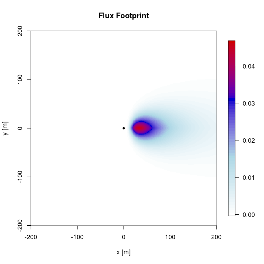
plot_flux_footprint(ffp_KM,xlim=c(-0,500),ylim=c(0,500)) #different time step and rotated according to wind direction
7.3 Flux footprint climatology
Flux footprint climatologies can be created as composites of single flux footprints by averaging over several FFP calculations (with calc_flux_footprint_climatology for both discussed flux footprint models).
i=1:(dim(dat)[1]) #calculation takes some time
ffp_clim=calc_flux_footprint_climatology(zm=zm,ws_mean=dat$ws_mean[i],wd_mean=dat$wd_mean[i],L=L[i],
v_sd=dat$v_sd[i],ustar=ustar[i],method="KM2001",plot=FALSE)plot_flux_footprint(ffp_clim,xlim=c(-400,400),ylim=c(-400,400)) 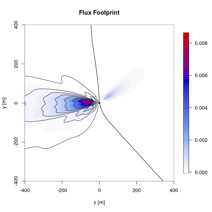
The flux footprint (climatology) can then be plotted on a digital elevation model (DEM), an aerial photo or an ecosystem type classification, see e.g. Kljun et al. (2015) therein Fig. 5 or Pirk et al. (2023) therein Fig. 4.
For Norway, you can download DEM data from geonorge.no, in particular the DTM10 dataset is suitable as flux footprint background (https://kartkatalog.geonorge.no/metadata/dtm-10-terrengmodell-utm33/dddbb667-1303-4ac5-8640-7ec04c0e3918).
References
Hsieh, C. I., G. Katul, and T. Chi. 2000. “An approximate analytical model for footprint estimation of scalar fluxes in thermally stratified atmospheric flows.” Advances in Water Resources 23 (7): 765–72. https://doi.org/10.1016/S0309-1708(99)00042-1.
Kljun, N., P. Calanca, M. W. Rotach, and H. P. Schmid. 2015. “A simple two-dimensional parameterisation for Flux Footprint Prediction (FFP).” Geosci Model Dev 8: 3695–3713. https://doi.org/10.5194/gmd-8-3695-2015.
Kormann, R., and F. X. Meixner. 2001. “An analytical footprint model for non-neutral stratification.” Boundary-Layer Meteorol 99: 207–24.
Pirk, N., K. Aalstad, Y. A. Yilmaz, A. Vatne, A. L. Popp, P. Horvath, A. Bryn, et al. 2023. “Snow-Vegetation-Atmosphere Interactions in Alpine Tundra.” Biogeosciences 20: 2031–47. https://doi.org/10.5194/bg-20-2031-2023.